
In this Python tutorial we will explore how to create a Density Plot using the Matplotlib Graphing Library. We will discuss a variety of different methods, each with it’s own unique twist. But before that, what exactly is a Density plot?
A density plot is a representation of the distribution of a numeric variable. We typically use Density plots to observe how a certain variable’s values are distributed in the dataset. Density plots are actually a variation of Histograms, a more smoothed out version that makes it easier to observe the distribution.
Method#1 – Using Seaborn with Matplotlib
The bw in bw_method stands for “bandwidth”. This is a setting that determines how smooth the resulting density plot will be.
import matplotlib.pyplot as plt
import seaborn as sns
data = [7,2,3,3,9,0,1,1,2,3,1,2,0,7,1,5,5,2,1,8]
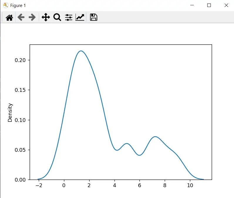
sns.kdeplot(data, bw_method=0.25)
plt.show()
Older versions of seaborn may use the bw parameter instead of bw_method. This is now deprecated, and may be discontinued in future releases, so switch to using bw_method instead.
bw_method accepts both strings and scalar values. It’s default value is “scott” which makes it use an equation known as Scott’s Rule. You may wish to adjust this value however, or use alternative equations according to your data for an accurate density plot.
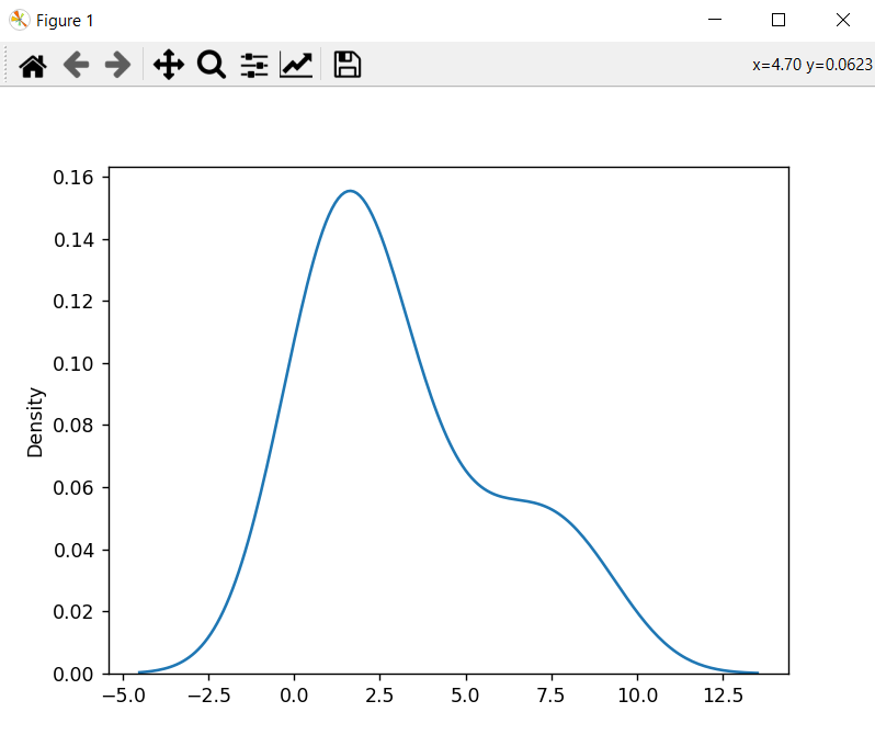
Here is the graph when using the default values for bw_method:
Method#2 – Using SciPy with Matplotlib
Another library that we can use to generate our density plot is SciPy. This library is in-fact being used in the background for many other libraries, such as Seaborn for computing distributions.
import matplotlib.pyplot as plt
import numpy as np
from scipy.stats import kde

data = [7,2,3,3,9,0,1,1,2,3,1,2,0,7,1,5,5,2,1,8]
density_function = kde.gaussian_kde(data, bw_method=0.3)
x = np.linspace(-2, 10, 300)

plt.plot(x, density_function(x))
plt.show()
The output for the above code:
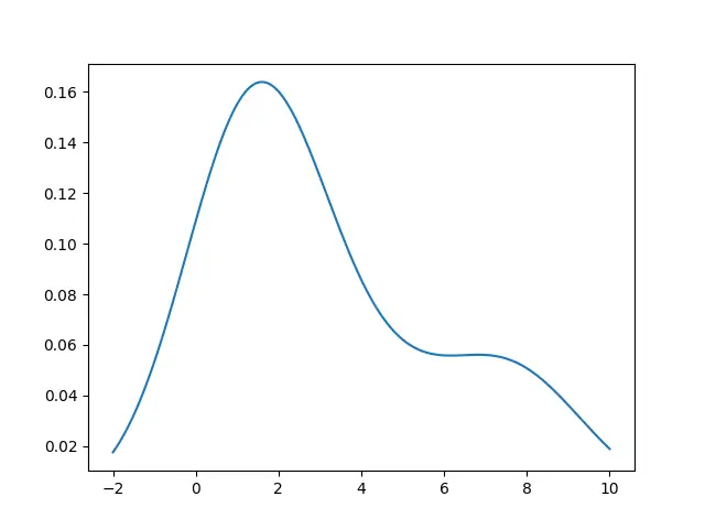
This may vary from dataset to dataset, but SciPy is generally faster than the other methods mentioned in this tutorial.
Method# 3 – Using Pandas
We can also use the Pandas library with Matplotlib to generate a Density plot.
import matplotlib.pyplot as plt
import pandas as pd
data = [7,2,3,3,9,0,1,1,2,3,1,2,0,7,1,5,5,2,1,8]
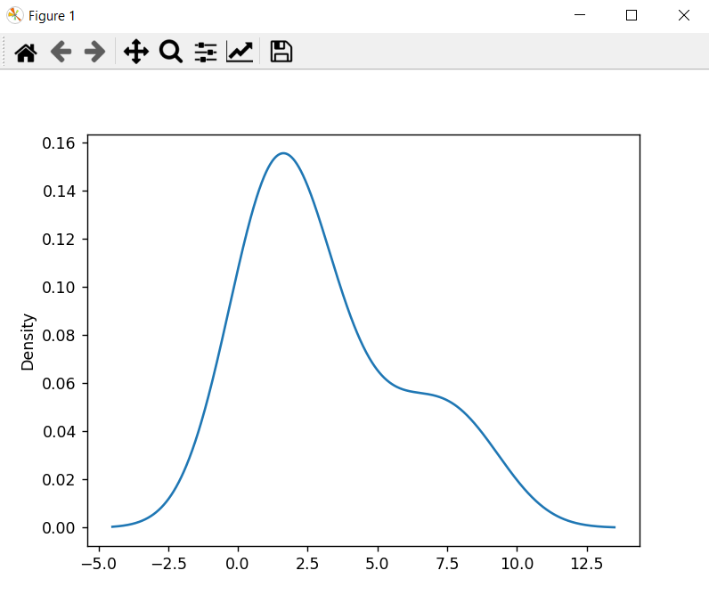
pd.Series(data).plot(kind='density')
plt.show()
You can also adjust the bandwidth here by passing in the bw_method parameter with an appropriate value.
import matplotlib.pyplot as plt
import pandas as pd

data = [7,2,3,3,9,0,1,1,2,3,1,2,0,7,1,5,5,2,1,8]
pd.Series(data).plot(kind='density', bw_method=0.5)
plt.show()
Method# 4 – Seaborn distplot
distplot is a special function inside that can create various types of graphs based off the parameters passed to it.
import matplotlib.pyplot as plt
import seaborn as sns
import pandas as pd

data = [7,2,3,3,9,0,1,1,2,3,1,2,0,7,1,5,5,2,1,8]
sns.distplot(data, kde_kws={'bw_method': 0.3})
plt.show()
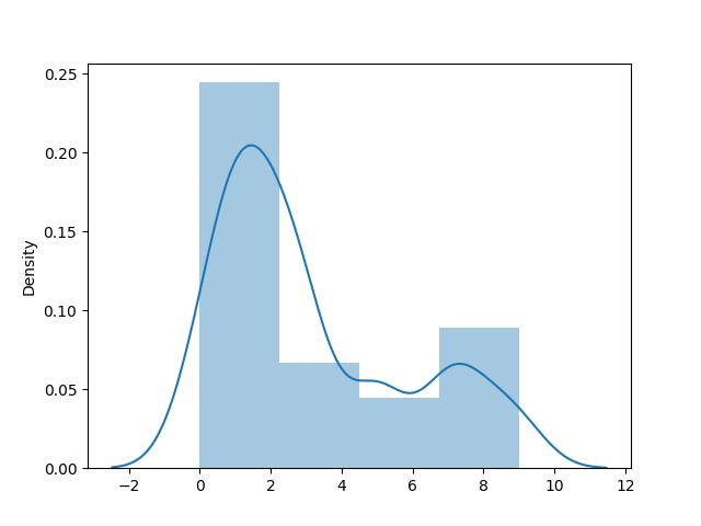
Passing in kde=false will disable the density plot. Likewise, passing in hist=true will disable the histogram. By default both of these true, so we can see both a density plot and histogram in the above output.
This marks the end of the Density Plot with Matplotlib in Python Tutorial. Any suggestions or contributions for CodersLegacy are more than welcome. Questions regarding the tutorial content can be asked in the comments section below.